![]()
get the data
run the following two cells below to get the data for this exercise, then followup by reading the questions and writing your own code to answer them.
!pip install requests
### important: this code downloads the data for you into "adult.data" csv file in the current directory
import requests

url = "http://mlr.cs.umass.edu/ml/machine-learning-databases/adult/adult.data"
request = requests.get(url)
request.raise_for_status()
with open('adult.data', 'w') as f:
    f.write(request.text)

### now the data is available in the csv file adult.data.
### read the questions below
# import pandas as pd
# pd.read_csv('adult.data')
income for adults from the 1994 census
This dataset was extracted done by Barry Becker from the 1994 Census database. source: http://mlr.cs.umass.edu/ml/datasets/Adult
Listing of attributes:
- age: continuous.
- workclass: Private, Self-emp-not-inc, Self-emp-inc, Federal-gov, Local-gov, State-gov, Without-pay, Never-worked.
- fnlwgt: continuous.
- education: Bachelors, Some-college, 11th, HS-grad, Prof-school, Assoc-acdm, Assoc-voc, 9th, 7th-8th, 12th, Masters, 1st-4th, 10th, Doctorate, 5th-6th, Preschool.
- education-num: continuous.
- marital-status: Married-civ-spouse, Divorced, Never-married, Separated, Widowed, Married-spouse-absent, Married-AF-spouse.
- occupation: Tech-support, Craft-repair, Other-service, Sales, Exec-managerial, Prof-specialty, Handlers-cleaners, Machine-op-inspct, Adm-clerical, Farming-fishing, Transport-moving, Priv-house-serv, Protective-serv, Armed-Forces.
- relationship: Wife, Own-child, Husband, Not-in-family, Other-relative, Unmarried.
- race: White, Asian-Pac-Islander, Amer-Indian-Eskimo, Other, Black.
- sex: Female, Male.
- capital-gain: continuous.
- capital-loss: continuous.
- hours-per-week: continuous.
- native-country: United-States, Cambodia, England, Puerto-Rico, Canada, Germany, Outlying-US(Guam-USVI-etc), India, Japan, Greece, South, China, Cuba, Iran, Honduras, Philippines, Italy, Poland, Jamaica, Vietnam, Mexico, Portugal, Ireland, France, Dominican-Republic, Laos, Ecuador, Taiwan, Haiti, Columbia, Hungary, Guatemala, Nicaragua, Scotland, Thailand, Yugoslavia, El-Salvador, Trinadad&Tobago, Peru, Hong, Holand-Netherlands.
- income: >50K, <=50K.
import pandas as pd
from IPython.display import display
import matplotlib.pyplot as plt
import seaborn as sns
import numpy as np
%matplotlib inline
sns.set()
1. load the data
- extract the column names from the description and read the csv while supplying the columns names
- rename columns with a hyphen
-to use underscores_insead. example:capital-gain --> capital_gain
- rename columns with a hyphen
description = """\
age: continuous.
workclass: Private, Self-emp-not-inc, Self-emp-inc, Federal-gov, Local-gov, State-gov, Without-pay, Never-worked.
fnlwgt: continuous.
education: Bachelors, Some-college, 11th, HS-grad, Prof-school, Assoc-acdm, Assoc-voc, 9th, 7th-8th, 12th, Masters, 1st-4th, 10th, Doctorate, 5th-6th, Preschool.
education-num: continuous.
marital-status: Married-civ-spouse, Divorced, Never-married, Separated, Widowed, Married-spouse-absent, Married-AF-spouse.
occupation: Tech-support, Craft-repair, Other-service, Sales, Exec-managerial, Prof-specialty, Handlers-cleaners, Machine-op-inspct, Adm-clerical, Farming-fishing, Transport-moving, Priv-house-serv, Protective-serv, Armed-Forces.
relationship: Wife, Own-child, Husband, Not-in-family, Other-relative, Unmarried.
race: White, Asian-Pac-Islander, Amer-Indian-Eskimo, Other, Black.
sex: Female, Male.
capital-gain: continuous.
capital-loss: continuous.
hours-per-week: continuous.
native-country: United-States, Cambodia, England, Puerto-Rico, Canada, Germany, Outlying-US(Guam-USVI-etc), India, Japan, Greece, South, China, Cuba, Iran, Honduras, Philippines, Italy, Poland, Jamaica, Vietnam, Mexico, Portugal, Ireland, France, Dominican-Republic, Laos, Ecuador, Taiwan, Haiti, Columbia, Hungary, Guatemala, Nicaragua, Scotland, Thailand, Yugoslavia, El-Salvador, Trinadad&Tobago, Peru, Hong, Holand-Netherlands.
"""

columns = [line.split(':')[0] for line in description.splitlines()] + ['income']
columns = [column.replace('-', '_') for column in columns]
columns
df = pd.read_csv('adult.data', names=columns)
df.head()
2. look at the head, info, dtype, check for nan values
df.info()
> answer:
no null values. yippee!
3. what are the value counts of the categorical variables: workclass, education, marital_status, occupation, relationship, race, sex, native_country, income?
- do you notice the extra space ‘ ‘ at the beginning of each value?
- remove the extra space
for column in "workclass education marital_status occupation relationship race sex native_country income".split():
    print(column, ':')
    print(df[column].value_counts())
    print()
for column in "workclass education marital_status occupation relationship race sex native_country income".split():
    print(column, ':')
    df[column] = df[column].str.strip()
    print(df[column].value_counts())
    print()
4. turn ‘sex’ and ‘income’ into 0/1 fields
- replace the categorical ‘sex’ column with a numerical ‘female’ column with value 1 for females and 0 for males
- replace the categorical ‘income’ column with a numerical ‘over50k’ column with value 1 for ‘>50k’ and 0 for ‘<50K’
df.rename(columns={'sex': 'female', 'income' : 'over50k'}, inplace=True)
df.replace({'female' : {'Male' : 0, 'Female' : 1 }, 'over50k' : {'>50K' : 1, '<=50K' : 0}}, inplace=True)
df.head(10)
5. use .describe() function to get descriptive statistics for most columns
- make sure that ‘sex’ and ‘over50k’ are now numerical fields
df.describe()
2. explore capital gains / losses
capital_gain
- plot the histogram for capital gains
- verbally describe what you see
sns.distplot(df.capital_gain, kde=False)
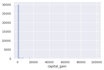
> answer:
almost everyone has $capital_gains=0$
2. for people who have capital_gain > 0 - plot the histogram for capital gains
sns.distplot(df[df.capital_gain > 0].capital_gain, kde=False)
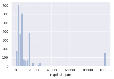
> remark:
what’s this weird bump at $100K ?
3. how many people have capital gains over 25000?
- use
value_counts()to look at all the values of capital_gain over 25000. - what’s weird about the data?
df[df.capital_gain > 25000].capital_gain.value_counts()
> answer:
- the values seem oddly perscriptive… why do specific value repeat so much, and no values in between?
- are the values here coding for something?
- also 99999 is maybe a cap value of capital gains?
4. could the people who had capital_gain==25124 be related?
df[df.capital_gain == 25124]
> answer:
- very unlikely, 3 widows and 1 never-married are unlikely to share one household.
- their “shared” capital_gain either codes for something, or is some kind of quantized property of a calculated field, or other fluke
5. does capital_gain over 50k mean income is over 50k?
df[df.capital_gain > 50000].over50k.mean()
> answer:
- 100% of people who had capital_gain>50000 had income over 50k
- so inspite of the weirdness we saw in the values, we can probably keep and interpret this variable as intended
capital_loss
- plot the histogram of capital_loss
sns.distplot(df.capital_loss, kde=False)
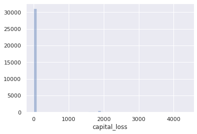
> remark
again we see almost everybody having 0 capital losses
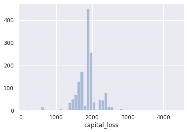
2. for people who have capital_loss > 0
- plot the histogram for capital_loss
sns.distplot(df[df.capital_loss !=0].capital_loss, kde=False)
3. how many people had both capital_gain>0 and capital_loss>0 ?
len(df[(df.capital_gain > 0) & (df.capital_loss >0)])
4. who can afford to lose money on capital investments?
- what percent of people overall had over 50K income?
- what percent of people with 0 capital_loss? with capital_loss>0?
print("proportion of people who earn over 50K:\n{}".format(df.over50k.mean()))
print()
print("proportion of people who earn over 50K, by capital_loss > 0:")
print(df.groupby(df.capital_loss >0).over50k.mean())
sns.barplot(x="lost_capital", y="over50k", data=df.assign(lost_capital=df.capital_loss >0))
plt.axhline(y=df.over50k.mean(), linestyle="--")
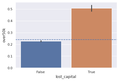
> answer:
- having capital_loss > 0 is correlated with earning more than 50K.
- in fact, the proportion of over50k is twice as large in capital losers than in the general population
combining and binning
- create a new capital_change column that equals capital_gain - capital_loss
df = df.assign(capital_change=df.capital_gain - df.capital_loss)
df.head()
sns.barplot(
    y="has_capital_change",
    x="over50k",
    data=df.assign(has_capital_change=df.capital_change.abs() > 0)
    )

2. use the qcut function to quantize/bin/cut capital_change into a new columns called capital_change_bin with 10 bins of equal proportions.
- do not bin capital_change==0 values as there are too many of them
- to simplify using this column later, use the left side of the interval created as the label
- label rows with capital_change==0 as having capital_change_bin=0
- make sure you have no null values for capital_change_bin
# do not bin capital_change==-0
capital_change_bins = pd.qcut(df[df.capital_change !=0].capital_change, 10)

# use left side of interval as label
capital_change_bins = capital_change_bins.apply(lambda interval: interval.left)

# add capital_change_bin to df
df['capital_change_bin'] = capital_change_bins

# look at the last 4 columns
df.iloc[:, -4:].head()
# label rows with capital_change==0 as having capital_change_bin=0
df.replace({'capital_change_bin' : {np.nan : 0}}, inplace=True)

# look at the last 4 columns
df.iloc[:, -4:].head()
# make sure you have no null values for capital_change_bin
df.capital_change_bin.isnull().sum()
3. how many people have a non-zero capital_change?
- lets call this ‘has_capital_change’
- plot ‘has_capital_change’ over ‘over50k’
- what do you learn from this diagram?
sns.barplot(
    y="has_capital_change",
    x="over50k",
    data=df.assign(has_capital_change=df.capital_change.abs() > 0)
    )
plt.grid(True)
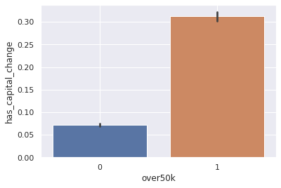
> answer:
- for people earning less than 50K, only ~7.5% try to have “money work for them” in terms of capital gain/loss
- for people earning above 50K, over 30% have non-zero capital change
4. plot capital_change by over50k
- what do you learn from this diagram
sns.barplot(x='over50k', y='capital_change', data=df)
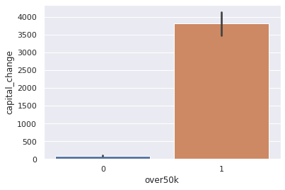
> answer:
- people earning over50k had the means/knowledge/opportunity to invest in capital, and earned a mean ~3500$ from capital
5. plot over50k by capital_change_bin
- what can you learn from this diagram?
bars = sns.lineplot(x='capital_change_bin', y='over50k', data=df)
plt.setp(bars.get_xticklabels(), rotation=90);
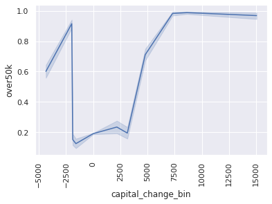
> answer:
- among people that has lost/earned roughly 2500$ or under in capital_change, there is very minor difference in proportion of over50K earnings relative to the general population
- however, among those that have earned or lost in excess of ~2500$ there is a sharp increase in the proportion of over50K earners
education
- what is the mean education_num by education?
- sort the education categories by the mean_values. does it make sense?
- check out other descriptive statistics to see if anything falls out of place
- turn education into a categorical ordered type
- plot education VS education_num
- what have we learned?
# - what is the mean education_num by education?
# - sort the education categories by the mean_values. does it make sense?
df.groupby('education').education_num.mean().sort_values()
> answer:
yes, makes sense. looks like
education_numis a numerical encoding foreducation
# - check out other descriptive statistics to see if anything falls out of place
df.groupby('education').education_num.describe()
> answer
- yes, we see that std is 0 and min=max.
- that means there are no deviations or wrong encodings in the data. yippee!
#   - turn education into a categorical ordered type
sorted_education = df.groupby('education').education_num.mean().sort_values().index.values
print(sorted_education)
df.education = df.education.astype(pd.CategoricalDtype(sorted_education, ordered=True))

#   - plot education VS education_num
bars = sns.barplot(x='education', y='education_num', data=df)
plt.setp(bars.get_xticklabels(), rotation=90);
plt.grid(True)

#   - what have we learned?
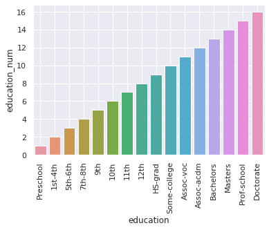
> answer:
we can now interchangably use either education_num or education in our graphs,
depending if we want to emphasize the categorical name of the education or numerical size
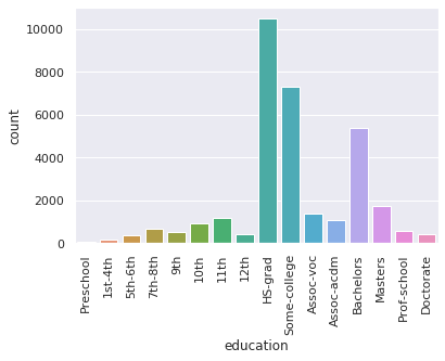
2. plot the distribution for education
bars = sns.countplot(df.education)
plt.setp(bars.get_xticklabels(), rotation=90);
3. plot over50k by education
- what do we learn?
bars = sns.barplot(y='over50k', x='education', data=df)
plt.setp(bars.get_xticklabels(), rotation=90);
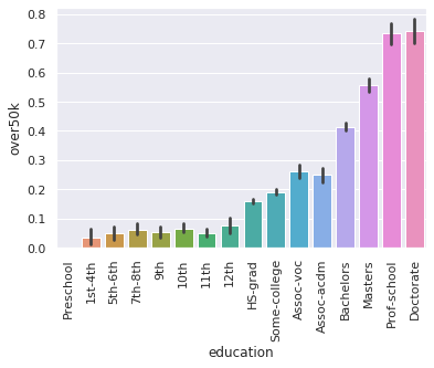
> answer:
- over50k seems to be stringly correlated with education,
- with significant improvements to outcomes at High School, Bachelors, Masters and Proffesional/Doctorate attainment levels
4. plot hours_per_week by education
- what can we learn?
- now use the hue=”over50k” of seaborn to see hours_per_week by education/over50k.
- learn anything else?
bars = sns.lineplot(y='hours_per_week', x='education', ci="sd", data=df)
plt.setp(bars.get_xticklabels(), rotation=90);
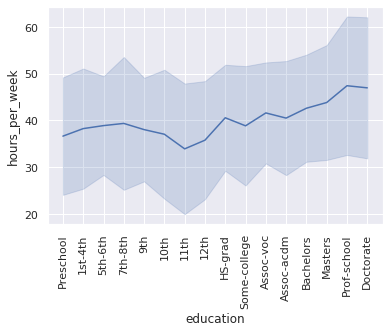
> answer:
- we observe High-School gradues to have roughly a 40-hour work week
- with education above highschool, we see a strong trend for more hours-per-week as education increases, above and beyond 40 hours
- we see a sharp decline in work hours for highschool dropouts (9th-12th grade education). perhaps indicative of physical/mental health issues or life circumstances that make work difficult.
- for education up until 8th grade we see a positive trend that more education allows for more work, reaching almost 40 hour weeks of full employment
bars = sns.lineplot(y='hours_per_week', x='education', hue='over50k', ci="sd", data=df)
plt.setp(bars.get_xticklabels(), rotation=90);
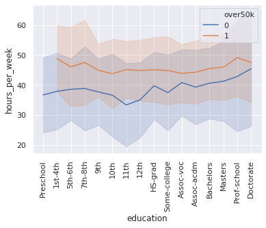
> answer:
- those that earn above 50K work approx 45 hours per week across most education levels. with exceptions being at low education levels (where sample sizes are small so confidence intervals are large) and for “Prof-School” education (doctors?), where the mean is closer to ~50 hour weeks.
- those that earn under 50K work less hours across almost all education levels, mostly around 40 hour weeks at above high-school level education (except perhaps those with Doctorates where sample sizes are small)
> note for later:
look further at relationship between hours worked and over50k
5. plot education_num by occupation
- sort by mean education_num
occupation_by_education = df.groupby("occupation").education_num.mean().sort_values().index.values
bars = sns.boxplot(
    x="occupation",
    y='education_num',
    order=occupation_by_education,
    data=df,
    # medianprops={"color":"white"},
    showfliers=False,
    showmeans=True
    )
_ = plt.setp(bars.get_xticklabels(), rotation=90)
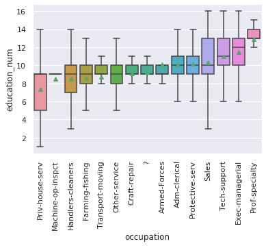
> remark:
clearly there seems like 5 cluster of jobs by education level:
- “Priv-house-serv” (servants)
- “Machine-op-inspect” to “Arned forced” (blue collar)
- “Adm-clerical” to “sales” (white collar)
- “Tech-support” - “Exec-managerial” (tech / management)
- “Prof-specialty” (doctors/lawyers/proffesionals)
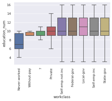
6. plot education_num by workclass
- sort by mean education_num
workclass_by_education = df.groupby("workclass").education_num.mean().sort_values().index.values
bars = sns.boxplot(x="workclass", y='education_num', order=workclass_by_education,  showfliers=False, data=df)
_ = plt.setp(bars.get_xticklabels(), rotation=90)
7. create a crosstab or a pivot_table of education VS occupation.
- normalize it by the education rows (each row X shows the conditional probability of having occupation Y by education level X)
- create a heatmap that shows which occpupations are most likely for each education level
- verbally describe what you’ve learned
occ_by_edu_df = pd.crosstab(
    df.education,
    df.occupation.astype(pd.CategoricalDtype(occupation_by_education, ordered=True)),
    normalize='index')

fig, ax = plt.subplots(figsize=(7,7))

sns.heatmap(
    occ_by_edu_df
    , robust = True
    , ax=ax
    , cmap="Oranges"
    , linewidths=.75
);
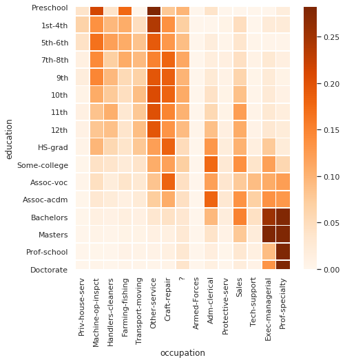
> answer:
the heatmap shows for each education/row, which occupations are most likely to be taken by individuals with that education attainment.
- for the very lower end of education, “machine-op-inspect” or “farming-fishing” is likely
- Those with high-school or below attainment, are likely to find themselves in the large “Other-service”, “Craft-repair” or “transport-moving” occupations, since these are large overall.
- mid-level education “some-college” to “assoc-acdm” find a wide range of horizontal occuptions
- for Bachelor and above education “Exec-managerial” and “Prof-specialty” are highly likely
8. create a crosstab or a pivot_table of education VS workclass.
- normalize it by the education rows (each row X shows the conditional probability of having workclass Y by education level X)
- create a heatmap that shows which workclass is most likely for each education level
- verbally describe what you’ve learned
- re-run this analysis without the private sector
class_by_edu_df = pd.crosstab(
    df.education,
    df.workclass.astype(pd.CategoricalDtype(workclass_by_education, ordered=True)),
    normalize='index')

fig, ax = plt.subplots(figsize=(7,7))

sns.heatmap(
    class_by_edu_df
    , robust = True
    , ax=ax
    , cmap="Oranges"
    , linewidths=.75
);
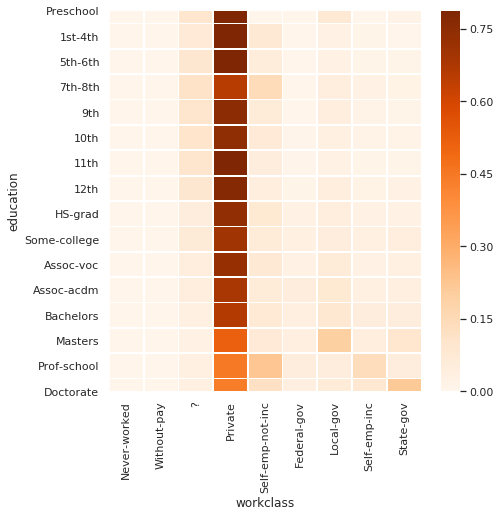
> answer:
almost everyone, regardless of education, works in the private sector. yippee!
non_private_df = df[df.workclass != 'Private']

class_by_edu_df = pd.crosstab(
    non_private_df.education,
    non_private_df.workclass.astype(pd.CategoricalDtype(workclass_by_education, ordered=True)),
    normalize='index')

fig, ax = plt.subplots(figsize=(7,7))

sns.heatmap(
    class_by_edu_df
    , robust = True
    , ax=ax
    , cmap="Oranges"
    , linewidths=.75
);
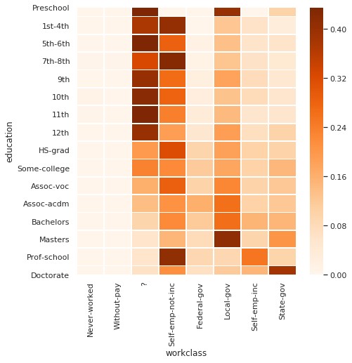
> answer:
outside the private sector:
- those with lowest education, mostly are unclassified by workclass, or are self-employed
- high scool grads tend to be self-employed
- mid-level education tend to be self-employed or local-government
- people with masters degree tend to be employed by local goverment
- people with prof-school tend to be self-employed
- people with doctorates tend to be employed by state-government
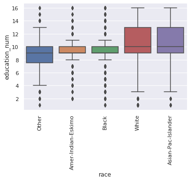
9. plot “race” vs “education_num
race_by_education = df.groupby('race').education_num.mean().sort_values().index.values
bars = sns.boxplot(x="race", y="education_num",  order=race_by_education, data=df)
_ = plt.setp(bars.get_xticklabels(), rotation=90)
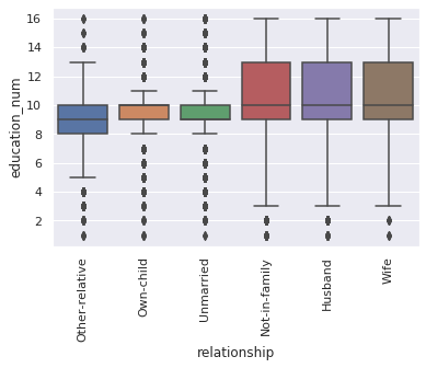
10. plot “relationship” vs “education_num
rel_by_education = df.groupby('relationship').education_num.mean().sort_values().index.values
bars = sns.boxplot(x="relationship", y="education_num",  order=rel_by_education, data=df)
_ = plt.setp(bars.get_xticklabels(), rotation=90)
occupation / workclass
- how many levels of occupation?
print(df.occupation.nunique())
print(df.occupation.unique())
2. how many levels of worklass?
print(df.workclass.nunique())
print(df.workclass.unique())
3. how many combinations? potential? actual?
print("potential:", df.workclass.nunique() * df.occupation.nunique())
print("actual:", len(df.groupby(['occupation', 'workclass'])))
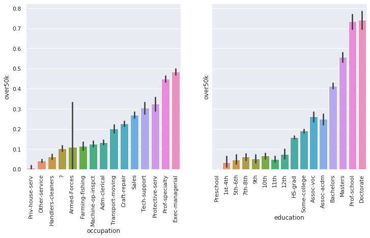
4. plot over50k by occupation
- sort by mean over50k
- compare this to over50k by education. which variable more strongly predicts income?
- compare tjos to education_num by occupation. are the highest paying jobs correlated with highest earning education?
fig, axs = plt.subplots(ncols=2, sharey=True, figsize=(12,6))
occ_by_50k = df.groupby('occupation').over50k.mean().sort_values().index.values
bars = sns.barplot(x='occupation', y='over50k', order=occ_by_50k, data=df, ax=axs[0])
plt.setp(bars.get_xticklabels(), rotation=90);

bars = sns.barplot(x='education', y='over50k', data=df, ax=axs[1])
plt.setp(bars.get_xticklabels(), rotation=90);
fig, axs = plt.subplots(ncols=2, sharex=True, figsize=(12,6))
bars = sns.barplot(x='occupation', y='over50k', order=occ_by_50k, data=df, ax=axs[0])
plt.setp(bars.get_xticklabels(), rotation=90);

bars = sns.barplot(x='occupation', y='education_num', ci="sd", order=occ_by_50k, data=df, ax=axs[1])
plt.setp(bars.get_xticklabels(), rotation=90);
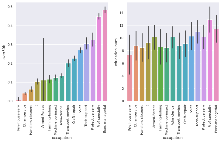
> answer:
- education looks like a stronger indicator of income, because disparities in income are higher when grouped by education than when grouped by occupation
- the highest paying occupations are not the same as the occupations requiring highest education. perhaps this is due to education needs varying wildly within occupations
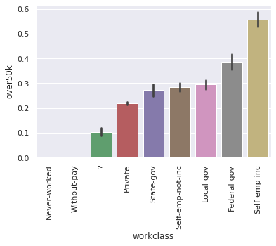
5. plot over50k by workclass
class_by_50k = df.groupby('workclass').over50k.mean().sort_values().index.values
bars = sns.barplot(x='workclass', y='over50k', order=class_by_50k, data=df)
plt.setp(bars.get_xticklabels(), rotation=90);
6. look at combinations of occupation / workclass
- what are the top combinations in terms of earning over50k? how many people in that category?
occupation_class = df.groupby(['occupation', 'workclass']) \
    .over50k.agg(["mean", "count"]) \
    .sort_values(by="mean", ascending=False)

occupation_class.head(10)
2. how many of these combinations have more than 100 people?
occupation_class = occupation_class[occupation_class['count'] > 100]
print(len(occupation_class))
occupation_class.head(10)
3. show a heatmap
of the mean over50k of occupation-vs-worklass for combinations with more than 100 people. center the heatmap at the populations mean over50k for increased effect. what conclusions can you draw?
sns.heatmap(
    occupation_class['mean'].unstack(1)
    , center=df.over50k.mean()
    , robust = True
    , linewidths=.75)
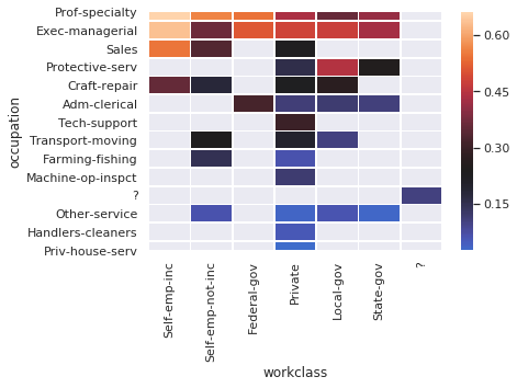
> answer:
- Prof-speciality and Exec managerial lead the earners across all work classes.
- Self-employed-inc (having your own firm incorporated) is great
- the private sector often has worse over50k mean than other sectors for the same occupations
- Protective-serv (police/firemen) working for local-gov is a sweet deal
7. create a numerical encoding for occupation / workclass pairs
- create a new column called “occ_class” that combines the string of the occupation and workclass
- use the library category_encoders, here’s an intro how to do it
- use the weight of evidence encoder
ce.woe.WOEEncoderhere’s an article explaining it - add the encoded occ_class as a new column called
occ_class_woeto your dataframe
!pip install category_encoders
# pip install category_encoders
import category_encoders as ce

def get_occupation_workclass(person):
    occupation, workclass = person['occupation'], person['workclass']
    if (occupation, workclass) in occupation_class.index:
        return f"{occupation}|{workclass}"
    else:
        return "other"

df['occ_class'] = df.apply(get_occupation_workclass, axis=1)
ce_target = ce.woe.WOEEncoder(cols = ['occ_class'])
ce_target.fit(df["occ_class"], df['over50k'])
df["occ_class_woe" ] = ce_target.transform(df["occ_class"], df['over50k'])

# show the encoding
df.groupby("occ_class")['occ_class_woe'].max().sort_values()
correlations
- which features are most important, which correlate?
- compute the correction matrix of features with themselves
corr = df.corr()
corr.head()
2. draw a clustermap of this correlation
- center the cluster at 0
- annotate the plot with the correlation values
sns.clustermap(corr,
               linewidths=.75,
               annot=True,
               fmt=".2f",
               center=0
               )
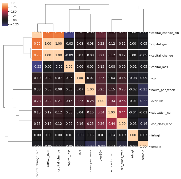
3. look at the strongest correlations and draw some conclusions.
> answer:
we obviously ignore the diagonal where variables have 100% correlation with themselves
- a strong .44 correlation between
education_numandocc_class_woeis especially interesting because we encoded occupation/class toward theover50kvariable, but received a stronger correlation with education than with income (at a smaller .36). this shows that education is a super strong determinant of occupation/class, and that occupation/class determines income- at a slighly lower .34,
education_numis still very strongly correlated withover50k, showing education is key for higher incomes- at .28
capital_change_binis strongly correlated withover50k. it is my belief that here causality goes backwards - higher incomes create capital investments, rather than the opposite. perhpas an indication for that is that capital_change_bin is not strongly correlated with anything butover50k- at .25
occ_class_woeis strongly correlated withhours_per_week. stronger than the .15 correlation ofeducation_numwithhours_per_week, and we’ve seen analysis that with higher education people work more hours. it appears that higher education enables higher paying jobs, with require more hours.- at .23
hours_per_weekis strongly correlated withover50k. this is probably explained by the previous item. better jobs require more hours, rather than the more obvious more hours worked creating higher salary.- at -0.23
hours_per_weekis strongly negatively correlated with beingfemale. so women work less hours. this is only slightly more negative than the -0.22 correlation women have withover50k. are women earning less because they are not willing to work as many hours? there is no definitive answer here, but it is interesting to also note the -0.16 negative correlation ofocc_class_woewith being female, so they might be choosing lower paying jobs with shorter hours. lastly, it is interesting to note the correlation offemaleandeducation_numis a negligble -0.01, that is women have the same levels of education as men.- the strongest correlation is
capital_change_binandcapital_gainbut that is an artifact of how we built that variable.